
Statistical learning refers to a vast set of tools for understanding data. These tools can be classified as supervised or unsupervised. It is a framework for machine learning drawn from fields of statistics and functional analysis. This deals with the problem of finding a predictive function based on data. In supervised learning, a statistical model is used to predict an output based on one or more inputs. On the other hand, in unsupervised learning there are no supervising output for the inputs. From such data, relationships and structures are learnt and used for predictions.
Shehroz Khan, ML Researcher of University of Toronto has a very fitting example to explain this. “You go bag-packing to a new country, you did not know much about it - their food, culture, language etc. However, from day 1, you start making sense there, learning to eat new cuisines including what not to eat, find a way to that beach etc.
Scenario1 is an example of supervised classification, where you have a teacher to guide you and learn concepts, such that when a new sample comes your way that you have not seen before, you may still be able to identify it.
Scenario2 is an example of unsupervised classification, where you have lots of information but you did not know what to do with it initially. A major distinction is that, there is no teacher to guide you and you have to find a way out on your own. Then, based on some criteria you start churning out that information into groups that makes sense to you.”
In a typical setting, the input variables are denoted by X with a subscript to distinguish them. These variables go by various names like features, predictors, independent variables or simply variables. The output variable (also called as response or dependent variables) is often denoted by the symbol Y.
Suppose a response Y is given out by p different predictors, X1, X2, X3,… Xp such that there is some relationship between Y and X = (X1, X2, X3,… Xp), then the relationship can be written in a general form :
$Y = f(X) + ϵ$
Here f is some fixed but unknown function of X1,…, Xp and ϵ is a random error term which is independent of X and has a mean zero.
- Why should one estimate f?
- How to estimate f?
- Parametric Methods
- Non-Parametric Methods
- Prediction Accuracy – Model Interpretability Trade Off
- Supervised vs Unsupervised Learning
- Regression vs Classification Problems
- References
Why should one estimate f?
Prediction
In many situations, a set of inputs X are readily available, but the output Y cannot be easily obtained. In this condition as the error term averages to zero, we can predict Y by using $\hat{Y}$ = $\hat{f}(X)$ where $\hat{f}$ represents our estimate for f and $\hat{Y}$ represents the resulting prediction for Y. In this setting, $\hat{f}$ is often treated as a black box, in the sense that one is not typically concerned with the exact form of $\hat{f}$, if it yields accuracte predictions for Y.
The accuracy of $\hat{Y}$ as a prediction for Y depends on two quantities, generally called the reducible error and the irreducible error. In general, $\hat{Y}$ will not be a perfect estimate for f, and this inaccuracy will introduce some error. This error is reducible because we can potentially improve the accuracy of $\hat{f}$ by using the most appropriate statistical learning technique to estimate f. However, even if it were possible to form a perfect estimate for f, so that our estimated response took the form $\hat{Y}$ = $\hat{f}(X)$, our prediction would still have some error in it! This is because Y is also a function of ϵ, which, by definition, cannot be predicted using X. Therefore, variability associated with ϵ also affects the accuracy of our predictions. This is known as the irreducible error, because no matter how well we estimate f, we cannot reduce the error introduced by ϵ.
Why is the irreducible error larger than zero?
The quantity ϵ may contain unmeasured variables that are useful in predicting Y; since we don’t measure them, f cannot use them for its prediction. The quantity ϵ may also contain unmeasurable variation.
For a given estimate $\hat{f}$ and a set of predictors X, which yields the prediction $\hat{Y}$ = $\hat{f}(X)$. If both $\hat{f}$ and X are fixed, then the following result can be deduced.
$E(Y-\hat{Y})^2 = [f(X)-\hat{f}(X)]^2 + Var(ϵ)$
Here, $E(Y-\hat{Y})^2$ represents the expected value or average of the squared difference between the predicted and the actual value of Y. Var(ϵ) represents the variance associated with the error term ϵ. The first term on RHS of equation is the reducible error while the second term is the Irreducible error.
Inference
In order to understand how Y changes as a function of X1, X2, X3,… Xp , a few of the following things might help.
Which predictors are associated with the response – It usual that not all predictors are associated with the target Y, so its very important to identify which variables are useful.
What is the relationship between the response and each predictors – Some predictors tend to have positive relationship with Y, i.e. increasing the predictor increases the values of Y; and some predictors have negative relationship with Y. Depending on the complexity of f, the relationship of Y with a predictor might depend on values of other predictors.
Can the relationship be linear or complicated – In real life scenarios, the predictors don’t tend to have a linear relationship with the response and linear equations do not give an accurate representation of the relationship between input and output variables, so other non-linear relationships like logarithmic, etc need to be considered.
Sometimes the models can be a combination of both prediction and inference where some variables need to be inferred and others be predicted.
Though being simple and easily predictable, linear models do not always yield accurate predictions. In such situations, highly non-linear approaches give predictions with high accuracy but at an expense of not being interpretable easily.
How to estimate f?
To estimate f, some amount of observations are used to train the method being used in prediction. These observations are called training data. While the rest of the observations are used to predict the unknown outcome and are called as testing data.
Statistical learning methods are characterized as either parametric or non-parametric.
Parametric Methods
It involves two steps. First an assumption about functional form or shape of f is assumed.
e.g. if f(X) = β0 + β1X1 + β2X2 +…+ βpXp, i.e. if we assume that f is linear then instead of having to estimate an entirely arbitrary p-dimensional function f(X), only the p+1 coordinates β0, β1, …, βp need to be estimated.
In the second step, a model needs to be selected and then the training data is used to fit or train the model. In the case of linear model, the values of the parameters β0, β1, …, βp need to be found out such that Y ≈ β0 + β1X1 + β2X2 +…+ βpXp
The model based approach is referred as parametric as it reduces the problem of estimating f down to one of estimating a set of parameters. Assuming a parametric form for f simplifies the problem of estimating f because it is generally much easier to estimate a set of parameters, such as β0, β1, …, βp in the linear model, than it is to fit an entirely arbitrary function f. The potential disadvantage of a parametric approach is that the model chosen will usually not match the true unknown form of f. If the chosen model is too far from the true f, then the estimate will be poor. This problem can be addressed by choosing flexible models that can fit many different possible functional forms for f. But in general, fitting a more flexible model requires estimating a greater number of parameters. These more complex models can lead to a phenomenon known as overfitting the data, which essentially means they follow the errors, or noise, too closely.
Non-Parametric Methods
Non-parametric methods do not make explicit assumptions about the functional form of f. Instead they seek an estimate of f that gets as close to the data points as possible without being too rough or wiggly. Such approaches can have a major advantage over parametric approaches: by avoiding the assumption of a particular functional form for f, they have the potential to accurately fit a wider range of possible shapes for f. Any parametric approach brings with it the possibility that the functional form used to estimate f is very different from the true f, in which case the resulting model will not fit the data well. In contrast, non-parametric approaches completely avoid this danger, since essentially no assumption about the form of f is made. But non-parametric approaches do suffer from a major disadvantage: since they do not reduce the problem of estimating f to a small number of parameters, a very large number of observations (far more than is typically needed for a parametric approach) is required in order to obtain an accurate estimate for f.
Prediction Accuracy – Model Interpretability Trade Off
The methods being used are either restrictive (less flexible) or more flexible in nature. The restrictive methods can produce a small range of shapes to estimate f and vice versa. The restrictive methods are generally used for inference problems as they are more interpretable. e.g Understanding the results of a linear relationship would be easy as the relationship between Y and X1, X2, … Xp can be interpreted. Problems where prediction is the sole purpose is where the more flexible methods can be used. But the more flexible methods often tend to overfit hence its quite common to get accurate predictions with less flexible methods.
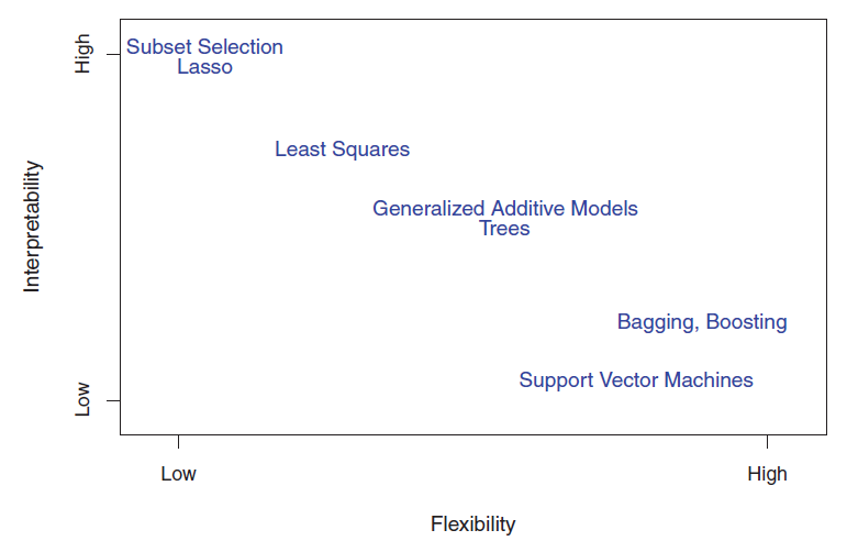
The above figure shows a tradeoff between flexibility and interpretability for some of the general ML methods.
Supervised vs Unsupervised Learning
Most statistical learning problems are categorized into either supervised or unsupervised.
The supervised learning problems have an associated response with each observation. Models are made to relate the response to the predictors with aim of accurately predicting the response of future observations or to understand the relationship between the response and the predictors for inference. Examples of this method is linear regression, logistic regression, boosting, SVM, etc.
The unsupervised learning problems have no associated response with the observations. So the relationships between the variables or the observations needs to be understood. One of the methods is clustering where the observations are put into distinct groups having same patterns found from the variables.
Another kind of learning method is semi-supervised learning where some observations have both predictor measurements and a response measurement and the remaining observations have a predictor measurement but no response measurement. Such situations can arise when the predictor measurement is an easy task but measurement of response is costly.
Regression vs Classification Problems
Variables are characterized as either quantitative or categorical. Quantitative variables take on numerical values while the categorical variables take on the qualitative values. e.g. A person’s age, weight, height is quantitative while his/her sex is categorical (Male/Female). Problems with quantitative response are called regression problems while those involved with categorical response are called as classification problems. Linear regression is used with regression problems but logistic regression is used with classification problems. Some methods like K-nearest neighbors can be used in either case.
References
- Statistical learning theory. (2017). En.wikipedia.org. Retrieved 10 June 2017, from https://en.wikipedia.org/wiki/Statistical_learning_theory
- Quora. (2017). Retrieved 10 June 10, 2017 from https://www.quora.com/What-is-the-difference-between-supervised-and-unsupervised-learning-algorithms
- James G., Witten D., Hastie T., Tibshirani R. (2013). An introduction to Statistical Learning. New York, NY: Springer
This article is written by ashmin Follow him @ashminswain.
Share this:


