Simple Linear Regression

• Simple Linear Regression
• The Coefficients
• Accuracy of the coefficient estimates
• Model Accuracy
• References

Simple Linear Regression

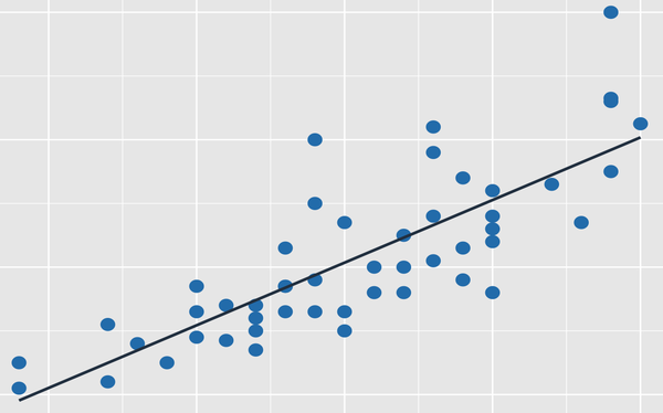
Simple Linear Regression is an approach for predicting a quantitative response Y on the basis of a single predictor variable X where it assumes that there is an approximate linear relationship between Y and X. Mathematically this can be represented as:

Y ≈ β₀ + β₁X

The “≈” is read as “is approximately modeled as” or simply Y getting regressed onto X. The β₀, β₁ are known as model coefficients or parameters. The training data is used to produce estimate $\hat{β_0}$ and $\hat{β_1}$ by computing

$\hat{y} = \hat{β_0} + \hat{β_1}x$

where $\hat{y}$ indicates prediction of Y based on X = x. The hat symbol ^ denotes the estimated value for an unknown parameter or coefficient.

The Coefficients

Let $\hat{y_i} = \hat{β_0} + \hat{β_1}x_i$ be the prediction for Y for the ith value of X. Then the difference between the ith observed response value and the ith response that is predicted by the linear model is the residual given by $e_i = y_i + \hat{y_i}$.

The residual sum of squares (RSS) is given as RSS = e₁² + e₂² + … + e_n² or simply by

$RSS = (y_1 - \hat{β_0} - \hat{β_1}x_1)^2 + (y_2 - \hat{β_0} - \hat{β_1}x_2)^2 + … + (y_n - \hat{β_0} - \hat{β_1}x_n)^2$

After some calculus, its proven that the least square coefficient estimates are

$\hat{β_1} = \frac{\sum_{i=1}^n (x_i-\bar{x})(y_i-\bar{y})}{\sum_{i=1}^n (x_i-\bar{x})^2}$

$\hat{β_0} = \bar{y} - \hat{β_1}\bar{x}$

where $\bar{y}$ and $\bar{x}$ are the sample means.

Accuracy of the coefficient estimates

With different data sets, the values of β₀, β₁ would change. Averaging the values over a large number of datasets would bring the value closer to the expected values.

$SE(\hat{β_0})^2 = \frac{1}{n} + \frac{\bar{x}^2}{\sum_{i=1}^n(x_i - \bar{x})^2}$

$SE(\hat{β_1})^2 = \frac{σ^2}{\sum_{i=1}^n(x_i - \bar{x})^2}$

Here SE is the standard error and σ is the standard deviation of each observation. Also σ² is the Var(ε). The formulas are valid if the errors ε_i for each of the observation are uncorrelated with the common variance σ². In general σ² is not known and is estimated from the data. This estimation is known as Residual Standard Error or RSE and is given by

$RSE = \sqrt{RSS/(n-2)}$.

The standard errors are used to estimate the confidence intervals. A 95% confidence interval is the range of values such that with 95% probability, the range will contain the true unknown of the parameter. For linear regression, the 95% confidence interval for β₁ takes the form $\hat{β_1}$ ± 2.SE($\hat{β_1}$) which is similar for $\hat{β_0}$ also.

t-statistics gives a measure of the standard deviations a value is away from 0 and is given by:

t = ($\hat{β_1}$ – 0)/ SE($\hat{β_1}$)

Probability of observing a value equal to |t| or larger assuming β₁ = 0 is called p-value. A small p-value indicates that it is unlikely to get a substantial association between the predictor and the response due to chance in absence of any real association between them. The small p-value gives an inference that there is an association between the predictor and the response. Typically p-values are desired to be below 5%.

Model Accuracy

The fit of linear regression is usually found by the RSE and R² statistics.

RSE is considered as a measure of the lack of fit of the model to the data. A large RSE denotes that model doesn’t fit the data well. As its not known what is a good RSE value, R2 statistics is used which takes a value between 0 to 1.

R² = 1 - (RSS/TSS) where TSS is the total sum of squares given by $\sum{(y_i - \bar{y})^2}$ and measures the total variance in the response before regression is performed. RSS gives the total variance in the response after the regression. So the R² statistic that is close to 1 indicates that a large proportion of the variability in the response has been explained by regression. A value closer to 0 means that the linear model is wrong or the error is high or both.

References

• James G., Witten D., Hastie T., Tibshirani R. (2013). An introduction to Statistical Learning. New York, NY: Springer