- Why a method other than logistic regression?
- Using Bayes Theorem for Classification
- Linear Discriminant Analysis for one predictor
- LDA for more than one predictors
- Quadratic Discriminant Analysis
- When to prefer LDA over QDA and vice versa?
- Comparison of Classification models
- References
Why a method other than logistic regression?
When the classes are well separated, the parameter estimates for logistic regression model is very unstable whereas LDA does not suffer from this problem.
With less number of observations and predictors have normal distribution, then LDA is again more stable than Logistic regression.
LDA is more popular for observations having more than two response classes.
Using Bayes Theorem for Classification
If an observation with K classes (K >= 2) needs to be classified, then the response variable can take on K possible distinct and unordered values. Let $π_k$ be the overall probability that a randomly chosen observation came from kth class i.e. the probability that a given observation is associated with the kth category of the response variable Y.
Let $f_k(X) \equiv Pr(X=x|Y=k)$ denotes the density function of X for an observation that comes from the kth class. $f_k(x)$ is relatively large if there is a large probability that an observation in the kth class has $X \approx x$ and $f_k(x)$ is small if it is very unlikely that an observation in the kth class has $X \approx x$.
Using Bayes Theorem,
$Pr(X=x | Y=k) = \frac{\pi_kf_k(x)}{\sum_{l=1}^K \pi_lf_l(x)}$
This suggest that instead of computing $p_k(x)$ which was used in logistic regression, the estimates of $\pi_k$ and $f_k(x)$ can be plugged into the above equations. Computing $\pi_k$ is easy if there is a random sample of responses from the population after which we compute the fraction of training observations that belong to kth class. Estimating $f_k(x)$ is challenging unless simple form of the densities is assumed.
Bayes classifier which classifies an observation to the class for which $p_k(x)$ is largest has the lowest possible error rate out of all classifiers, so $f_k(x)$ needs to be estimated to develop a classifier that approximates Bayes classifier.
Linear Discriminant Analysis for one predictor
For p = 1 i.e. one predictor, $f_k(x)$ needs to be estimated and put in the above equation in order to estimate $p_k(x)$. Observations can then be classified to the class where $p_k(x)$ is greatest. But first the form of $f_k(x)$ needs to be assumed. Suppose it is normal or Gaussian, then for one-dimension, the normal density is given by
$f_k(x) = \frac{1}{\sqrt{2\pi}\sigma_k}exp(-\frac{1}{2\sigma_k^2}(x-\mu_k)^2)$
Here $\sigma_k^2$ and $\mu_k$ are the variance and the mean of the kth class. Assuming $\sigma_k^2$ is the shared variance for all the k classes denoted by $\sigma^2$ and using it in the above equation for $p_k(x)$, its found that
$p_k(x) = \frac{\pi_k\frac{1}{\sqrt{2\pi}\sigma}exp(-\frac{1}{2\sigma^2}(x-\mu_k)^2)}{\sum_{l=1}^k\pi_l\frac{1}{\sqrt{2\pi}\sigma}exp(-\frac{1}{2\sigma^2}(x-\mu_l)^2)}$
Here $\pi_k$ is the prior probability that an observation belongs to kth class and is not equal to 3.14, the value of $\pi$.
The Bayes classifier involves assigning an observation X = x to the class for which the above equation is largest. So by taking the log of the equation and rearranging the terms, it is same as assigning the observation to the class for which
$\delta_k(x)=x.\frac{\mu_k}{\sigma^2}-\frac{\mu_k^2}{2\sigma^2} + log(\pi_k)$
is largest.
If X is drawn from a Gaussian distribution within each class, then the parameters $\mu_1,…, \mu_k, \pi_1,…, \pi_k$ and $\sigma^2$ need to be estimated. The LDA method uses the following estimates:
$\hat{\mu_k}=\frac{1}{n_k}\sum_{i:y_i=k}x_i$
$\hat{\sigma^2}=\frac{1}{n-K}\sum_{k=1}^K\sum_{i:y_i=k}(x_i-\hat{\mu_k})^2$
where n is the total number of training observations, $n_k$ is the number of training observations in the kth class. The estimate for $\mu_k$ is the average of all the training observations from the kth class whereas the estimate for $\sigma^2$ is the weighted average of the sample variances for each of the K classes. Plugging the estimates in the previous equation, an observation X = x is assigned to a class for which
$\hat{\delta_k}(x)=x.\frac{\hat{\mu_k}}{\hat{\sigma}^2}-\frac{\hat{\mu_k}^2}{2\hat{\sigma}^2}+log(\hat{\pi_k})$
is largest.
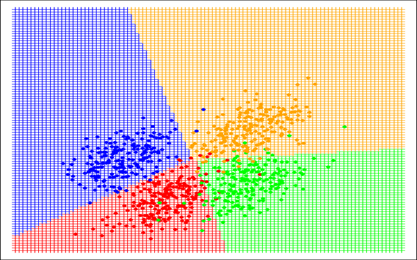
LDA for more than one predictors
To extend LDA classifier to multiple predictors, it can be assumed that X = $(X_1, X_2, …, X_p)$ is drawn from a multivariate Gaussian distribution with a class specific mean vector and a common covariance matrix. If $E(X) = \mu$ is the mean of X, the vector with p components and Cov(X) = $\sum$ is the p x p covariance matrix of X, the multivariate Gaussian density is given by
$f(x)=\frac{1}{(2\pi)^{p/2}|\sum|^{1/2}}exp(-\frac{1}{2}(x-\mu)^T\sum^{-1}(x-\mu))$
Plugging this value in the Bayes theorem and after a bit of algebra, its found that Bayes classifier assigns an observation X = x to the class for which
$\delta_k(x)=x^T\sum^{-1}\mu_k-\frac{1}{2}\mu_k^T\sum^{-1}\mu_k+log\pi_k$
is largest. The unknown parameters $\mu_1,…,\mu_k, \pi_1,…,\pi_k and \sum$ need to be estimated for this and they are similar to the values found for LDA for one predictor. $\delta_k(x)$ is a linear function of x. LDA decision rule depends on x only through a linear combination of its elements, hence the word Linear in LDA.
Quadratic Discriminant Analysis
The QDA classifier results from assuming that the observations from each class are drawn from a Gaussian distribution and plugging the estimates for the parameters into Bayes Theorem in order to perform prediction but unlike LDA, it assumes that each class has its own covariance matrix. Under this assumption, the Bayes classifier assigns an observation X = x to the class for which
$\delta_k(x)=-\frac{1}{2}x^T\sum_{k}^{-1}x+x^T\sum_{k}^{-1}\mu_k-\frac{1}{2}\mu_k^T\sum_{k}^{-1}\mu_k-\frac{1}{2}log|\sum_k|+log\pi_k$
is largest. The quantity x appears as a quadratic equation hence the name.
When to prefer LDA over QDA and vice versa?
The bias-variance tradeoff can be used to know when to use which method. With p predictors, estimating a covariance matrix requires estimating p(p+1)/2 parameters. QDA estimates covariance matrix for each class which is in total Kp(p+1)/2. The number of parameters hence become large. By instead assuming that the K classes share a common covariance matrix, the LDA model becomes linear in x so there are Kp linear coefficients to estimate. So LDA is a much less flexible classifier than QDA and so has less variance but higher prediction performance. If LDA’s assumption that K classes share a common covariance matrix is badly off, the LDA suffers from high bias. LDA tends to be a better method than QDA if the number of training observations are less so that reducing variance is important. QDA similarly is preferred if the training set is very large so that the variance of the classifier is not a major concern or if the assumption that the common covariance matrix for the K classes is weak.
Comparison of Classification models
As logistic regression and LDA vary only in their fitting procedures, the two methods give similar results. But LDA assumes that the observations are drawn from a Gaussian distribution with a common covariance matrix in each class, so it can outperform logistic regression if the assumption is correct and vice versa. KNN being a completely non-parametric approach, no assumptions are made about the shape of the decision boundary so it would outperform LDA and logistic regression when the decision boundary is highly non-linear but it doesn’t tell what predictors are important. As QDA assumes a quadratic decision boundary, it can accurately model a wider range of problems than the linear methods. It is not flexible as KNN but it can perform better in presence of a limited number of training observations as it doesn’t make any assumptions about the form of the decision boundary.
In a regression setting, a non-linear relationship between the predictors and the response can be accommodated by performing regression using transformations of the predictors. Similarly, for classification, transformation of predictors can be used to make logistic regression more flexible. This may not increase the performance depending on the increase of variance due to the added flexibility but would in turn reduce bias. The same can be done for LDA also and this new model can perform as well as QDA as it would include the quadratic terms and cross products.
References
- James G., Witten D., Hastie T., Tibshirani R. (2013). An introduction to Statistical Learning. New York, NY: Springer
This article is written by ashmin Follow him @ashminswain.
Share this:


